Grib Practice 03 (From the Starpath Grib School)
These practice exercises are best done after working those in Grib Practice 01. In both of these we use grib file GFS-sample-01.grb2. We use decimal Lat-Lon. N and E are positive. We use all true directions. Underway you may make other choices, or even use all compass on deck, and all true in the nav station. We will use all UTC for times, but underway you will have to go back and forth from UTC to ship's time.
You can use any Grib viewer for this exercise, XyGrib, qtVlm, OpenCPN, or the fine commercial products from LuckGrib and Expedition. Other nav programs such as Coastal Explorer or Time Zero also show grib files with convenient measurement tools. Don't forget the meteogram/meteotable option that many offer. Each Grib Viewer has its own way to set the forecast time to a specific value, but all let you do this. If you choose one of the free programs, then qtVlm has the most functionality for the type of analysis we cover in this exercise. For more practice, consider our online course in marine weather.
Check your answers with those at the end as you proceed.
(1) Let's look at some route planning for a Farr 40, located at (23.0, -145.0) on 2/23 at 12z, when our goal is to sail to the Pailolo Channel in HI at (21.1, -156.6). We are looking at the route ahead, starting from this intermediate position of the crossing.
(1a) After loading the grib file, what is the wind speed and direction at the starting time and location, and what is the bearing and distance to the destination in HI from this point?
Most grib viewers offer a way to measure range and bearing between points. We call this bearing the "rhumb line route" (RL).
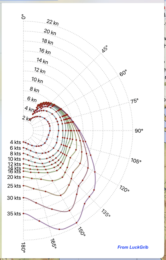
(1b) Look at the polar diagram and data for this boat in Figure 1 below (see our textbook on polar diagrams if needed). What is the dead downwind direction at the start time? If we assume the wind does not change, and assume we choose to sail directly toward the mark along the RL, what would be our TWA and resulting boat speed, and how long would it take to get there on that route at that speed?
(1c) Using the estimated speed from 1b, determine your estimated times and positions along the RL route at one-third and then two-thirds of the way there, and then advance the GFS forecast to those times to record the wind speed and direction at those points, and from that figure the TWA you would have in those winds if you were still sailing the RL heading. What might we conclude from what we find here?
In other words, figure where and when you will be one third and two thirds of the way there. Then read the winds at those times and places, and then figure TWAs using those wind directions and the RL heading of the vessel.
(1d) Let's now look into alternative routes on a more reaching heading. We will look at the two end points: Where we are now (at the start point above) and then we look in the vicinity of where we want to go. Let's assume that the winds we actually have as we read our instruments agree with the GFS forecasted winds we read from the Grib at the start time and place. This gives us some confidence in the forecasts—see, in passing, this note on Evaluating the Forecast.
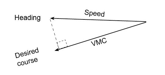
Looking at the existing wind at this start time and looking at the polar diagram for our boat (Figure 1 below), if we did not have other tactical reasons to do otherwise, what would be the heading that gave us the maximum speed toward our destination? So far we have discussed sailing directly toward the mark, but we know we can go faster by reaching more, but this means sailing farther, jibing back and forth. Is there a heading where the extra speed will make up for the extra distance we have to sail? In other words, what heading in this wind will yield the fastest speed in the direction of the mark, sometimes called "VMG course," and labeled VMC. (In NMEA terms, this is a parameter called Waypoint Closing Velocity, WCV, but we do not see that term in use much. It is computed by the navigation software, and programmers prefer VMC). This is not the same as VMG downwind that wind instruments read out directly, because our mark is not exactly downwind.
With that long intro, (1d) is this: in the starting wind conditions and known bearing to the mark, what does the polar tell us would be the heading we would take for the best VMC? Some navigation programs such as Expedition and qtVlm tell us the theoretical value of VMC directly, but without those tools we have to find it ourselves as we do in this exercise — in the real ocean we have to find it ourselves as well, even if we have software telling us what the theoretical values are. Real conditions do not often match the actual conditions. (The video solution shows the automated method.)
(1e) We can also, even more importantly, take a look at the anticipated winds during the approach to the final mark. Again referring to the polar in light of the winds forecasted at the approach (the final third figured above), what is the ideal heading we want to be on to make this approach, and in the forecasted wind pattern how early can we get onto that line. That is, what are the anticipated laylines as we approach the target? We want to draw these on the chart and navigate toward them... and keep monitoring any change in conditions that will rotate those lines.
[Background for this and earlier exercises is Modern Marine Weather, Section 7.2 on Using Weather Maps, specifically Figure 7.2-5 on setting up an approach cone, and Section 10.7 on Optimum Sailboat Routing.
The other real world factor we should highlight here is this winter time example has stronger winds than we are likely to meet in the summer and a prudent cruising sailboat with limited crew would be looking more to conservative routing in these conditions, not the optimum or fastest routing we are thinking about here. Again, this is just an exercise. These sustained 20+ kts are a definite handful for a small crew. With that said, in all circumstances all mariners have to keep an eye on the route down the line, not just at the moment.]
Knowing then how we might start out and how we should finish up, we can set about our route—and then monitor changes as we get new GFS wind forecasts every 6h along the way. We are doing this all manually. Later we will look into automated optimum route computations, where we let the computer do the thinking! You do not have to feel like the Lone Ranger if that thought gives pause for thought.
In a final summary: (1d) what is the best heading to start out on and very roughly how long might we hold it, and (1e) based on present forecast, what line on the chart do we want to be on when we approach the target and how early might we get onto it... if nothing were to change in the forecast?
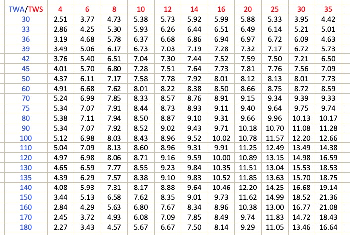
Figure 1. FARR 40 Polar data.
Download Farr40-374_polar.csv (semicolon separators, POL format as above)
Download Farr40-374_polar_Expedition.txt
Answers:
(1a) Wind at start time and position is 21 kts at 073. Bearing to the destination from this point is 262 T at a distance of 653 nmi.
(1b) Dead downwind would be 073 + 180 = 253 T. If we sail toward 262, this would be a starboard jibe, with a TWA of 171°—almost dead downwind. According to the polar we should make about 9.7 kts in these conditions, by interpolating the polar data [Note 1]. This would cover 653 nmi in 2d 20h 44m (68.7 hr). But this is not a good point of sail and the trade wind waves will be big on top of that in this pattern.
(1c) From 1b, the full route of 68.7 hr would be in thirds about 23h each, so first third occurs at 2/23 12z + 23h = 2/23 + 35h = 2/24 11z and the next third occurs on 2/24 11h + 23h = 2/24 34h = 2/25 10z. The distances covered would be 653/3 = 218 nmi per third. Thus the first third occurs when you are 435 nmi off, and the second third occurs when you are 218 nmi off.
Graphically or otherwise you can find that moving down the RL at 9.5 kts (not saying this is possible or a good choice) would put you at (22.446, -148.920) for the first third, which will happen on 2/24 11z with wind of 22.2 kts at 074. The second third occurs at (21.900, -152.258) on 2/25 10z with a wind of 21.9 kts at 087.
On a heading of 262, the stern is pointed toward 082, which puts the first third wind at TWA of 082-074 = 8° on starboard side, or TWA = 172 starboard, essentially where it was to start, just a bit closer to dead downwind. At the second third, we have 087 for the wind and 082 for the stern, so now the wind is 6° on the other side, for TWA 174 port.
In other words, this direct RL route from the start is essentially dead downwind and by the second third we either jibe or get jibed. In short, this was not a good route from the start, and we should look into more of a reaching angle, which as we shall see will be faster in any event. Dead downwind is always tricky to steer and especially bad in the big seas of persistently strong trade winds. We need to look into other routes.
(1d) Wind direction is 073, RL is 262, so the wind is on the starboard side and headed to the mark we are at TWA 171 (See 1b). From the polar data in Figure 1 (rounding TWS to 20 kts), we see that our fastest reaching angle downwind is about TWA 140 yielding a boat speed of 12.2. Downwind is 253 (TWA = 180), so to achieve TWA = 140 we need to come up 180-140 = 40°, which would be course 253+40 = 293. This would be the right course for the fastest boat speed at this wind speed, but not necessarily the fastest heading to get to our destination.
At this heading in 20 kts of wind we should sail at about 12.2 kts according to the polar, but we need to project that in the actual direction we want to go. At this point in the planning underway, it is actually easier and indeed more accurate to start looking at the nav instruments to see what VMC we are making at this new heading, but we can compute it, which we do in this exercise. In principle it is should be something like 12.2 x cos (293-262) = 10.5 kts.
So this is progress. We are moving at 12.2 kts, off course by 31°, but making good 10.5 to the mark—directly toward the mark we had only 9.7 kts. We are sailing away from the desired course line, so we have to jibe back at some point, and reevaluate everything on the other jibe. But this will be a faster course and more steady as it is not so dead downwind. But we are not done.
The reason we have to evaluate VMC is because we chose a heading for highest boat speed, and then just computed the VMC that that happened to give us; we did not choose a heading for optimum VMC. The curve of boat speed vs TWA has a fairly broad range of peak values, so we might find a better heading. Once we are, for example, trimmed up and sailing at heading 293, we then might try 5 or 10° higher and then 5 or 10° lower to see if we are optimized on the VMC—all nav software can compute and display the active value VMC, based on your target waypoint.
Also we should not be surprised al all in the real ocean if these values are different on the two jibes. The relative angle of wind and combined seas will often make one jibe favored over the other.
Again, this is easier on the boat than on a calculator, but we can mock it up in a spread sheet taking interpolated data from the polars, as shown below. Again, the video solution shows how to solve this automatically using qtVlm.
Here is what we might find from checking out the other headings, assuming the TWS was 20 kts (it was actually a bit higher at 21):
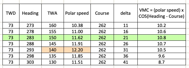
delta = Heading - Course
Namely, that whereas the fastest boat speed in 20 kts of wind is 12.2 kts at TWA 140, the optimum VMC will be at TWA 150 at 10.8 kts, which will be on heading 283. Our stern will be pointed toward 103; the wind is from 073, 30° onto the starboard quarter; 150° to the right of the bow. We have found this manually; see the video solution for a more direct result.
(1e) Now that we know in principle the headings we would follow, jibing back and forth as we head west, we can look ahead to see what we want when we get closer. This is the approach cone discussed in Figure 7.2-5 of the textbook. From 1c we learned that the wind for the last 218 nmi of the run was expected to be about 22 kts from at 087, and and then building to more like 25 at 090 to the finish. You can look at a meteogram plot of the winds at several places along the approach to confirm this. Note that we also have the NWS forecasts from the Honolulu office in HI as well as several buoys on this approach to check the GFS. By email request ask for PHZ180 to get the forecast out to 250 nmi. See textbook section 8.6.
At 25 kts we see from the polar that we have a peak speed of about 14.99 at TWA of about 150, so we can look at the target and draw in that TWA on the expected wind. With the wind at the end expected to be about 090, we would be on TWA 150 when on heading 90 + 150 = 240, which means we draw the layline away from the target at 240-180 = 060. If the winds evolve as expected, that is the line we want to be on.
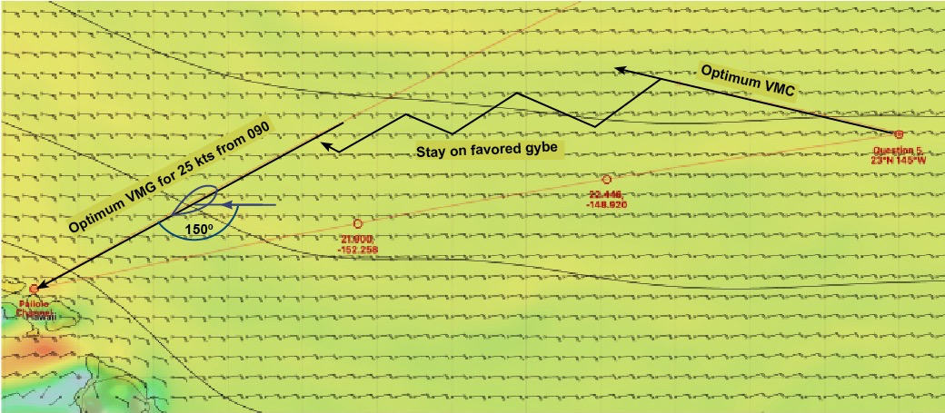
The summary is we figure best VMC and start off that way. At some point that jibe will no longer be favored and we have to jibe, back and forth, staying on favored jibe. This has to be continually watched and computed. The jibes here are just made up... but we could have guessed them with a lot of interpolation. At some early point (when you are confident about the approach forecast) look ahead to see winds at approach and figure approach line... which can rotate as the winds change, and we head for it. Generally you will have an approach cone to account for uncertainties. In our case, it looked like wind speed and angle were pretty steady over the last 3rd of the route.
A reminder that 25 kts of sustained wind is a strong wind to sail in for any sailor. Many sailors will rightfully be looking for more conservative points of sail, rather than optimum routes. This example was chosen at random in the winter, using live data when we started, so we just worked through it as if we have a boat full of experienced sailors on a well equipped boat.
____________
The above has been ways to think about a route all manually, just using the polar data and wind forecasts. Shortly we will add exercises on directly computing the optimum route using several navigation programs, where these intermediate steps are solved in a more systematic manner. This will be in Practice with Grib Files 04.
____________
Note 1. When I first worked this exercise i had a slightly different polar where this value was 9.5 kts, whereas using the better polar we have here now this is more like 9.7. But i will keep the 9.5 rather redo all the math. It does not matter for this analysis. This is just a note that you are not reading the polar data wrong.